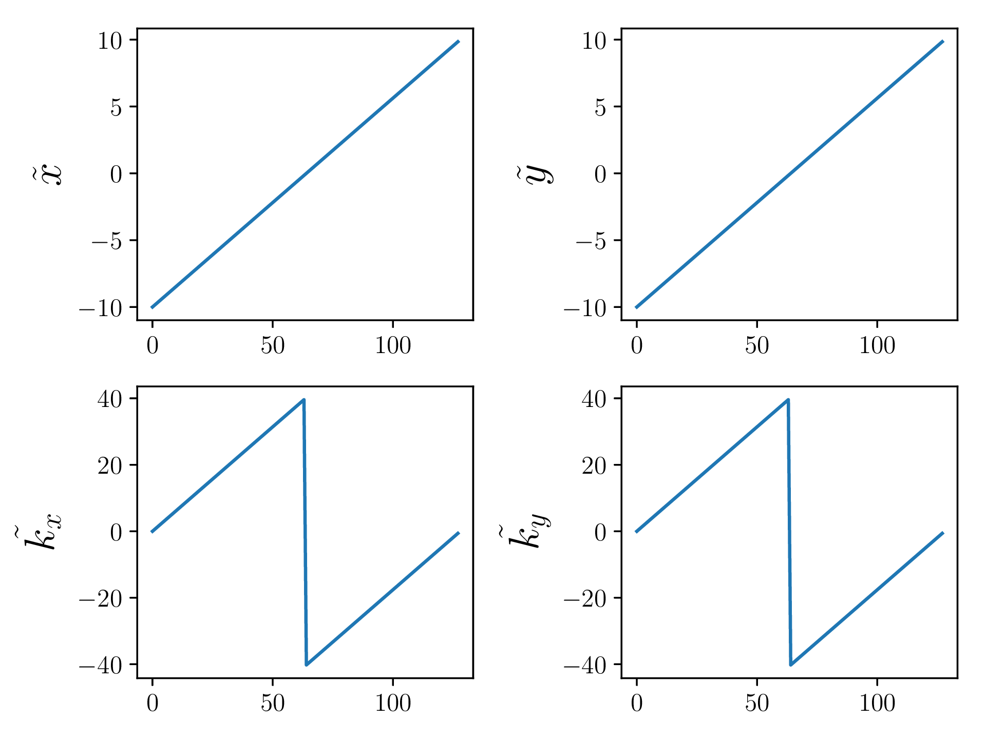
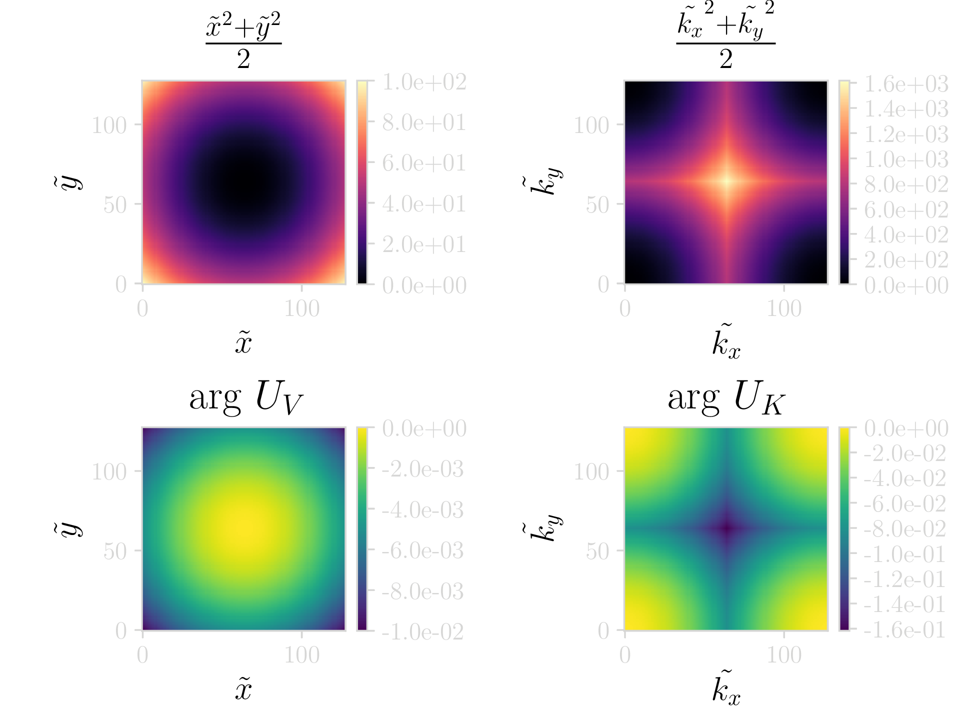
The following article is a work in progress, and will (hopefully) be updated over time. I will issue a RELEASE tag or similar when everything has been finished. Latest edit on 2018-12-30.
Q. How do available FFT routines compare over different libraries and accelerator hardware?
This is a question that I have wondered for some time, though it can be difficult for an apples-to-apples comparison. I will consider the above question in relation to the following project outline:
Comparing FFT implementations in a pseudospectral solver for linear and nonlinear Schrodinger equation dynamics
To decide on how to proceed, it is instructive to list (most of) the widely known and used FFT implementations.
Standard implementations
Following this link we can see that many FFT libraries and routines exist, for single node (single and multicore), as well as distributed implementations. For the purpose of this investigation we examine these codes that have:
- A publically available API.
- Well documented source and examples.
- Compilable and linkable across different architectures and compilers (GCC, Clang, MSVC).
[CPU]
- FFTW: http://fftw.org/ and https://github.com/FFTW/fftw3
- MKL-FFT: https://software.intel.com/en-us/articles/the-intel-math-kernel-library-and-its-fast-fourier-transform-routines
- clFFT: https://github.com/clMathLibraries/clFFT
- Eigen FFT (using kissfft backend): http://eigen.tuxfamily.org/index.php?title=EigenFFT
- sFFT: http://groups.csail.mit.edu/netmit/sFFT/code.html
- KFR FFT: https://github.com/kfrlib/fft
[GPU]
- cuFFT: http://docs.nvidia.com/cuda/cufft/index.html
- clFFT: https://github.com/clMathLibraries/clFFT
- fbfft: https://github.com/facebook/fbcuda/tree/master/fbfft and https://arxiv.org/abs/1412.7580
[Cutting edge]
The following tests will involve acquiring access to restricted resources, and may not even be feasible for the problem at hand due to differences in programmability and (in quantum hardware case) differences to interpretations of the results. As such, these will remain as potential options, until a time comes that either they are viable for testing, or deemed not applicable to the current problem.
- FPGA FFT (Xilinx and Altera/Intel): https://www.xilinx.com/products/intellectual-property/fft.html and https://www.altera.com/products/intellectual-property/ip/dsp/m-ham-fft.html
- Rigetti pyQuil quantum Fourier transform (QFT): http://pyquil.readthedocs.io/en/latest/getting_started.html
- IBM Qiskit Terra QFT: https://github.com/Qiskit/qiskit-terra/blob/master/examples/python/qft.py
Test cases
To ensure sufficient time is spent in the FFT routines I will opt for a 2D transform of an NxN grid, requiring N transforms, a transpose, and another N. The value of N can be scaled to determine sweet spots for all implementations. Granted, memory size will be the determining factor of how large we can go. $N=2^j$ where $j \in \mathbb{Z}, 7 \leq j \leq 11$ is a reasonable range of values to examine that should fit readily on most hardware.
For this, the following test precisions will be instructive:
- $\mathbb{C}2\mathbb{C}$ - 32-bit float (32-bits for each real and imaginary component)
- $\mathbb{C}2\mathbb{C}$ - 64-bit float
- $\mathbb{R}2\mathbb{C}$ - 32-bit float
- $\mathbb{R}2\mathbb{C}$ - 64-bit float
As a sample system to investigate, I will consider the case of a quantum harmonic oscillator (QHO). To investigate dynamics and their resulting accuracy, a known and analytically calculable result is useful. Generally, the use of 32-bit floats for this type of problem can be dangerous, as quantum states that are almost degenerate can fail to resolve to the lower of the states. Thus, it is best to use 64-bit floating point values for general cases, even though for toy problems 32-bit values can be fine (provided we take care). For this problem I will opt for a superposition state of the groundstate along the $xy$ plane, and the first excited state along $x$ with the groundstate along $y$. To put things more formally:
$$ \Psi(x,y) = \frac{ \Psi_{00}(x,y) + \Psi_{10}(x,y) }{\sqrt{2}}. $$ To construct the above wavefunction we will assume that the states $\Psi_{00}(x,y)$ and $\Psi_{10}(x,y)$ are outer products of the solutions to the QHO, as given by:
$$ \Psi_n(x) = \frac{1}{\sqrt{2^{n}n!}}\left(\frac{m\omega_x}{\pi\hbar}\right)^{\frac{1}{4}}\mathrm{e}^{-\frac{m\omega_x x^2}{2\hbar}}H_n(x), $$ where $$ H_n(x)=(-1)^n\mathrm{e}^{x^2}\frac{d^n}{dx^n}\left(\mathrm{e}^{-x^2}\right),$$ are the physicists’ Hermite polynomials. As we are looking for the ground and first excited states ($n=0,1$) we can simplify a lot of the above calculations: $H_0(x)=1$ and $H_0(x)=2x$. Next, we determine the states $\Psi_0(x)$ and $\Psi_1(x)$ as:
$$ \begin{eqnarray} \Psi_0(x) = \left(\frac{m\omega_x}{\pi\hbar}\right)^\frac{1}{4}\mathrm{e}^{-\frac{m\omega_x x^2}{2\hbar}},~ \Psi_1(x) = \frac{2x}{\sqrt{2}} \left(\frac{m\omega_x}{\pi\hbar}\right)^{\frac{1}{4}}\mathrm{e}^{-\frac{m\omega_x x^2}{2\hbar}}. \end{eqnarray} $$
Along a single dimension, our system can potentially be in any of the allowed harmonic oscillator states. Therefore, the overall state is given by a tensor product of the state along $x$ and that along $y$. If we assume the dimensionality of the Hilbert space along the $i$-th orthogonal spacial index is finite and given by $d_i$, then the overall system dimensionality (ie the total number of states we can consider) is $d = \displaystyle\prod_{i} d_i$.
Assuming an $n$-dimensional system, where each individual dimension is in the groundstate of the harmonic oscillator, we can define the tensor product state as $$ \Psi_n = \Psi_0^{\otimes n} = \Psi_0 \otimes \Psi_0 \cdots \otimes \Psi_0. $$
While the above is fine for a general case, for the purposes of FFTs we have assumed a much simpler system, dealing with combinations of only 2 states. We can then define them as $\Psi_{00}(x,y) = \Psi_{0}(x)\otimes\Psi_{0}(y)$ and $\Psi_{10}(x,y) = \Psi_{1}(x)\otimes\Psi_{0}(y)$. Thus, our final superposition state when filling everything in is given by $$ \Psi(x,y) = \left(\frac{m}{\pi\hbar}\right)^{\frac{1}{2}}\left(\omega_x\omega_y\right)^{\frac{1}{4}}\mathrm{e}^{-\frac{m}{2\hbar}\left(\omega_x x^2 + \omega_y y^2\right)}\left(x + \frac{1}{\sqrt{2}}\right). $$
To simplify life, I will assume some of the above quantities are set to unity (i.e. $m=\omega_x = \omega_y = \hbar = 1$). This will not change the dynamics of the simulation, but simplify the equations and the numerical implementation, which can help with improving accuracy. The above equation then becomes $$ \Psi(x,y) = \left(\frac{1}{\pi}\right)^{\frac{1}{2}}\mathrm{e}^{-\frac{1}{2}\left( x^2 + y^2 \right)}\left(x + \frac{1}{\sqrt{2}}\right). $$
For a more detailed explanation and approach to the above have a look at Christina Lee’s (albi3ro) blog post on time evolution, which will cover the method I use next.
To be continued
/***

This document will implement the quantum simulation aspects of the code, in as simple a means as possible.

***/
#include<stdio.h>
#include<stdlib.h>
#include<math.h>

#define GRIDSIZE 128
#define GRIDMAX 5
#define PI 3.14159
#define DT 1e-4


//################################################//

struct double2{
    double x;
    double y;
};

//Define the grid on which the simulation will be run.
struct Grid{
    double *x = (double*) malloc(GRIDSIZE*sizeof(double));
    double *y = (double*) malloc(GRIDSIZE*sizeof(double));
    double *xy2 = (double*) malloc(GRIDSIZE*GRIDSIZE*sizeof(double));

    double *kx = (double*) malloc(GRIDSIZE*sizeof(double));
    double *ky = (double*) malloc(GRIDSIZE*sizeof(double));
    double *kxy2 = (double*) malloc(GRIDSIZE*GRIDSIZE*sizeof(double));

    double2 *wfc = (double2*) malloc(GRIDSIZE*GRIDSIZE*sizeof(double2));
    double2 *U_V = (double2*) malloc(GRIDSIZE*GRIDSIZE*sizeof(double2));
    double2 *U_K = (double2*) malloc(GRIDSIZE*GRIDSIZE*sizeof(double2));
};

void setupGrids(Grid *grid){
    double invSqrt2 = 1/sqrt(2);
    //Position space grids
    for (int j=0; j < GRIDSIZE; ++j){
        grid->x[j] = -GRIDMAX + j*(2*GRIDMAX)/((double)GRIDSIZE);
        grid->y[j] = grid->x[j];
    }
    for(int i=0; i < GRIDSIZE; ++i){
        for(int j=0; j < GRIDSIZE; ++j){
            grid->xy2[j+GRIDSIZE*i] = 0.5*(grid->x[i]*grid->x[i]+grid->y[j]*grid->y[j]);
            //Evolution operator in position space
            grid->U_V[j+GRIDSIZE*i].x = cos(-grid->xy2[j+GRIDSIZE*i]*DT);
            grid->U_V[j+GRIDSIZE*i].y = sin(-grid->xy2[j+GRIDSIZE*i]*DT);

            //Wavefunction
            grid->wfc[j+GRIDSIZE*i].x = sqrt( 1/PI )*exp( -0.5 * ( grid->x[i]*grid->x[i] + grid->y[j]*grid->y[j] ) ) * ( grid->x[i] + invSqrt2 );
            grid->wfc[j+GRIDSIZE*i].y = 0.;
        }
    }

    //Momentum space grids
    for (int j=0; j < GRIDSIZE; ++j){
        grid->kx[j] = (j<(GRIDSIZE/2)) ? j*2*PI/(GRIDMAX) : -(GRIDSIZE - j)*(2*PI/(GRIDMAX));
        grid->ky[j] = grid->kx[j];
    }
    for(int i=0; i < GRIDSIZE; ++i){
        for(int j=0; j < GRIDSIZE; ++j){
            grid->kxy2[j+GRIDSIZE*i] = 0.5*(grid->kx[i]*grid->kx[i]+grid->ky[j]*grid->ky[j]);

            //Evolution operator in momentum space
            grid->U_K[j+GRIDSIZE*i].x = cos(-grid->kxy2[j+GRIDSIZE*i]*DT);
            grid->U_K[j+GRIDSIZE*i].y = sin(-grid->kxy2[j+GRIDSIZE*i]*DT);
        }
    }
}

//################################################//
int fileIO(Grid *grid){
    //Open files to write
    FILE *f_x = fopen("x", "w");
    FILE *f_y = fopen("y", "w");
    FILE *f_xy2 = fopen("xy2", "w");
    FILE *f_kx = fopen("kx", "w");
    FILE *f_ky = fopen("ky", "w");
    FILE *f_kxy2 = fopen("kxy2", "w");
    FILE *f_U_V = fopen("U_V", "w");
    FILE *f_U_K = fopen("U_K", "w");
    FILE *f_wfc = fopen("wfc", "w");

    //No safety checks because I'm a bad person

    fwrite(grid->x, sizeof(double), GRIDSIZE, f_x);
    fwrite(grid->y, sizeof(double), GRIDSIZE, f_y);
    fwrite(grid->xy2, sizeof(double), GRIDSIZE*GRIDSIZE, f_xy2);
    fwrite(grid->kx, sizeof(double), GRIDSIZE, f_kx);
    fwrite(grid->ky, sizeof(double), GRIDSIZE, f_ky);
    fwrite(grid->kxy2, sizeof(double), GRIDSIZE*GRIDSIZE, f_kxy2);
    fwrite(grid->U_V, sizeof(double2), GRIDSIZE*GRIDSIZE, f_U_V);
    fwrite(grid->U_K, sizeof(double2), GRIDSIZE*GRIDSIZE, f_U_K);
    fwrite(grid->wfc, sizeof(double2), GRIDSIZE*GRIDSIZE, f_wfc);

    //No moar opin

    fclose(f_x); fclose(f_y); fclose(f_xy2); fclose(f_kx);  fclose(f_ky);
    fclose(f_kxy2); fclose(f_U_V); fclose(f_U_K); fclose(f_wfc);
    return 0;
}

//################################################//
int main(){
    Grid grid;
    setupGrids(&grid);
    fileIO(&grid);
}


//################################################//


